Code coverage using a dynamic symbolic execution

Introduction

Code coverage is mainly used in the vulnerability research area. The goal is to generate inputs which will reach different parts of the program’s code. Then, if an input makes the program crash, we check if the crash can be exploited or not. A lot of methods exist to perform code coverage - like random testing or mutation generation - but in this short blog post, we will focus on code coverage using a dynamic symbolic execution (DSE) and explain why it’s not a trivial task. Please, note that covering up the code doesn’t mean finding every possible bugs. Some bugs do not make the program crash and this talk from slides 35 to 38 explains why. However, if we perform model checking associated with code coverage, it starts to get interesting =).

Code coverage and DSE

Note that unlike a SSE (static symbolic execution), a DSE is applied on a trace and can discover new branches only if these ones are reached during the execution. To go through another path, we must solve one of the last branch constraints discovered from the last trace. Then, we repeat this operation until all branches are taken.

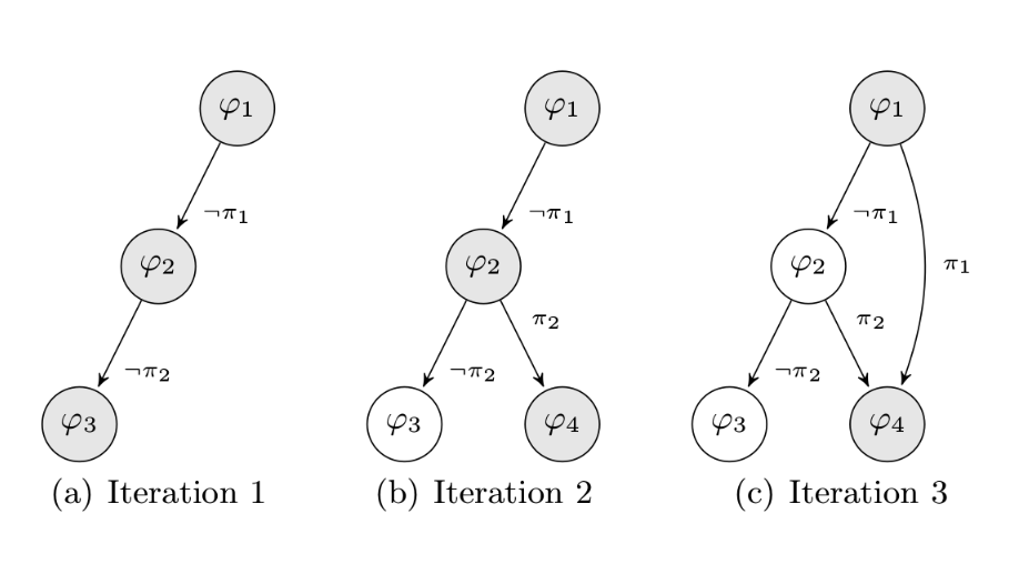
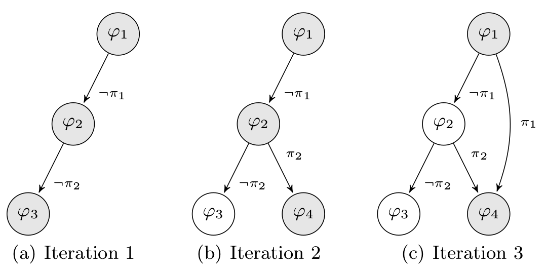
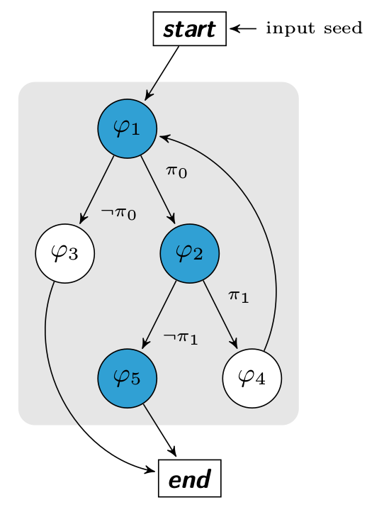
For example, let’s assume a program $P$ which takes an input called $I$, where I may be a model $M$ or a random seed $R$. An execution is denoted $P(I)$ and returns a set of constraints $PC$. All $\varphi_{i}$ represent basic blocks and $\pi_i$ represent the branches constraint. A model $M_i$ is (at least) one valid solution of a constraint $\pi_i$. For example, $M_1 = Solution(\neg\pi_1 \land \pi_2)$. To discover all paths, we maintain a worklist denoted $W$ which is a set of $M$.

At the first iteration, $I = R, W = \emptyset$ and $P(I) \rightarrow PC$. Then, $\forall \pi \in PC, W = W \cup { Solution(\pi) }$ and we execute once again the program such that $\forall M \in W, P(M)$. When a model $M$ is injected in the program’s input, it is deleted from the worklist $W$. Then, we repeat this operation until $W$ is empty.

Symbolic code coverage implies some pros and cons. For us, it is really useful when we work on a obfuscated binary. Indeed, applying symbolic coverage can detect opaque predicates or unreachable code but also repair a flattened graph (we will release soon another blog post about Triton and o-llvm). The worst con about the symbolic execution is when your expressions are too complexes which implies a timeout from the SMT solver or an impressive memory consumption (in the past, our bigger symbolic expression has consumed ~450 Go of RAM before timeout). This scenario mainly occurs when we analyse real large binaries or obfuscated binaries which contain polynomial functions. Some of these cons may partially be fixed by optimizing symbolic expressions but this subject will be another story to come later :).

Performing code coverage using Triton

Since the version v0.1 build 633 (commit 474fe2), Triton integrates everything we need to perform code coverage. These new features allow us to deal and compute the SMT2-Lib representation over an AST. In the rest of the blog post, we will focus on the design and the algorithm used to perform code coverage.

Algorithm

As an introduction (and to not turn our brain upside down), let assume this following sample of code which comes from the samples directory.

char *serial = "\x31\x3e\x3d\x26\x31";
int check(char *ptr)
{
  int i = 0;
  while (i < 5){
    if (((ptr[i] - 1) ^ 0x55) != serial[i])
      return 1;
    i++;
  }
  return 0;
}

Basically, this function checks if the input is equal to elite, and returns 0 if it is true, otherwise it returns 1. The control flow graph of this function is described below. It’s an interesting first example, because to cover all basic blocks we need to find the good input.

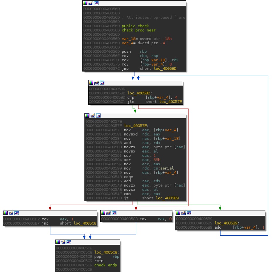
We can see that only one variable can be controlled, the one located at the address rbp+var_18 which refers to the argv[1] ’s pointer. The goal is to reach all the basic blocks in the function check by computing the constraints and using the snapshot engine until that every basic blocks are reached. For instance, the constraint to reach the basic block located at the address 0x4005C3 is [rbp+var_4] > 4 but we do not control this variable directly. In the other hand, the jump at the address 0x4005B0 depends on the user input and this constraint can be solved by performing a symbolic execution.

The algorithm which generalizes the previous idea is based on the Microsoft’s fuzzer algorithm (SAGE) and the next diagram represents our check function with its constraints. The start and end nodes represent respectively the function’s prologue (0x40056D) and the function’s epilogue (0x4005C8).

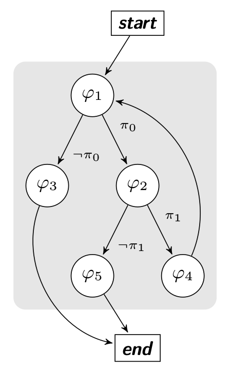
Before the first execution, we know nothing about branches’ constraints. So, as explained in the previous chapter, we inject some random seeds to collect the first $PC$ and build our set $W$. The trace of the first execution $P(I)$ is represented by the basic blocks in blue.

This execution gives us our first path constraint $P(I) \rightarrow (\pi_0 \land \neg \pi_1)$.

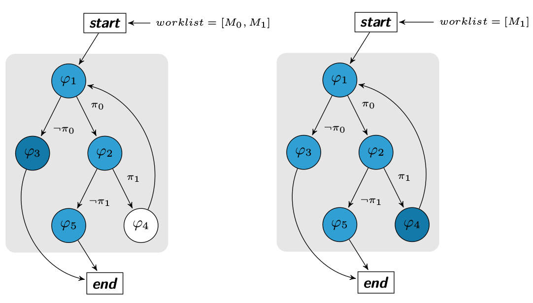
Based on our first trace, we know that there are two branches ($\pi_0 \land \neg \pi_1$) discovered and so 2 others undiscovered. To reach the basic bloc $\varphi_3$, we compute the negation of the first branch constraint. If and only if the solution $Solution(\neg \pi_0)$ is SAT, we add the model to the worklist W.

Same for $\varphi_4$ such that $W = W \cup {Solution(\pi_0 \land \neg(\neg \pi_1))}$. Once all solutions have been generated and models added to the worklist, we execute every models from the worklist.

Implementation

One condition to perform code coverage, is to predict the next instruction address when we are on a jump instruction. This condition is necessary to build the path constraint.

We can not put a callback after a branch instruction because the RIP register has already changed. As Triton creates semantics expressions for all registers, the idea is to evaluate RIP when we are on a branch instruction.

In a first time, we have developed a SMT evaluator to compute the RIP but we saw a little bit later that Pin provides IARG_BRANCH_TARGET_ADDR and IARG_BRANCH_TAKEN which can be used to know the next RIP values. With Pin, computing the next address is very easy, nevertheless the SMT evaluator was useful to check instruction’s semantics.

To perform the evaluation, we implemented the visitor pattern to transform the SMT abstract syntax tree (AST) to a Z3 AST. This design can be used to transform our SMT AST into any others representations.

The Z3 AST is easier to handle and can be evaluated or simplified with Z3 API. The transformation is performed by src/smt2lib/z3AST.h and src/smt2lib/z3AST.cpp.

We will now explain how the code coverage’s tool works. Let’s assume that inputs come from command’s line. Firstly, we have:

199
200
201
202
203

def run(inputSeed, entryPoint, exitPoint, whitelist = []):
  ...

if __name__=='__main__':
  TritonExecution.run("bad !", 0x400480, 0x40061B, ["main", "check"]) # crackme_xor

At line 176, we define the input seed bad ! which is the first program’s argument (argv[1]). Then, we give the address from the beginning of the code coverage (start block) - it’s at this address that we will take a snapshot. The third argument matches with the end block - it’s at this address that we will restore the snapshot. Finally, we can set a whitelist to avoid specific functions like library’s functions, cryptographic’s function and so on.

134
135
136
137
138
139
140
141
142
143
144
145
146
147
148
149
150
151
152
153
154
155

def mainAnalysis(threadId):

  print "[+] In main"
  rdi = getRegValue(IDREF.REG.RDI) # argc
  rsi = getRegValue(IDREF.REG.RSI) # argv

  argv0_addr = getMemValue(rsi, IDREF.CPUSIZE.QWORD)      # argv[0] pointer
  argv1_addr = getMemValue(rsi + 8, IDREF.CPUSIZE.QWORD)  # argv[1] pointer

  print "[+] In main() we set :"
  od = OrderedDict(sorted(TritonExecution.input.dataAddr.items()))

  for k,v in od.iteritems():
      print "\t[0x%x] = %x %c" % (k, v, v)
      setMemValue(k, IDREF.CPUSIZE.BYTE, v)
      convertMemToSymVar(k, IDREF.CPUSIZE.BYTE, "addr_%d" % k)

  for idx, byte in enumerate(TritonExecution.input.data):
      if argv1_addr + idx not in TritonExecution.input.dataAddr: # Not overwrite the previous setting
          print "\t[0x%x] = %x %c" % (argv1_addr + idx, ord(byte), ord(byte))
          setMemValue(argv1_addr + idx, IDREF.CPUSIZE.BYTE, ord(byte))
          convertMemToSymVar(argv1_addr + idx, IDREF.CPUSIZE.BYTE, "addr_%d" % idx)

The next code being executed is the mainAnalysis callback, we inject values to the inputs selected (line 148, 154) and we convert these inputs as symbolic variables (line 149, 155).

All inputs selected are stored in a global variable called TritonExecution.input. Then, we can begin the code exploration.

58
59
60
61

if instruction.getAddress() == TritonExecution.entryPoint and not isSnapshotEnabled():
  print "[+] Take Snapshot"
  takeSnapshot()
  return

When we are at the entry point, we take a snapshot in order to replay code exploration with a new input.

63
64
65
66
67
68
69
70
71
72
73
74

if instruction.isBranch() and instruction.getRoutineName() in TritonExecution.whitelist:

  addr1 = instruction.getAddress() + 2                # Address next to this one
  addr2 = instruction.getOperands()[0].getValue()     # Address in the instruction condition

  # [PC id, address taken, address not taken]
  if instruction.isBranchTaken():
    TritonExecution.myPC.append([ripId, addr2, addr1])
  else:
    TritonExecution.myPC.append([ripId, addr1, addr2])

  return

This test above checks if we are on a branch instruction like (jnz, jle …) and if we are in a function which is into the white list. If so, we get the two possible addresses (addr1 and addr2) and the effective address is computed by isBranchTaken() (line 69).

Then, we store into the path constraint the RIP expression, the address taken and the address not taken (line 73-76).

 81
 82
 83
 84
 85
 86
 87
 88
 89
 90
 91
 92
 93
 94
 95
 96
 97
 98
 99
100
101
102
103
104
105
106
107
108
109
110
111
112
113
114
115
116
117
118
119
120
121
122
123
124
125
126

if instruction.getAddress() == TritonExecution.exitPoint:
  print "[+] Exit point"

  # SAGE algorithm
  # http://research.microsoft.com/en-us/um/people/pg/public_psfiles/ndss2008.pdf
  for j in range(TritonExecution.input.bound, len(TritonExecution.myPC)):
    expr = []
    for i in range(0,j):
        ripId = TritonExecution.myPC[i][0]
        symExp = getFullExpression(getSymExpr(ripId).getAst())
        addr = TritonExecution.myPC[i][1]
        expr.append(smt2lib.smtAssert(smt2lib.equal(symExp, smt2lib.bv(addr,  64))))

    ripId = TritonExecution.myPC[j][0]
    symExp = getFullExpression(getSymExpr(ripId).getAst())
    addr = TritonExecution.myPC[j][2]
    expr.append(smt2lib.smtAssert(smt2lib.equal(symExp, smt2lib.bv(addr,  64))))


    expr = smt2lib.compound(expr)
    model = getModel(expr)

    if len(model) > 0:
        newInput = TritonExecution.input
        newInput.setBound(j + 1)

        for k,v in model.items():
            symVar = getSymVar(k)
            newInput.addDataAddress(symVar.getKindValue(), v)
        print newInput.dataAddr

        isPresent = False

        for inp in TritonExecution.worklist:
            if inp.dataAddr == newInput.dataAddr:
                isPresent = True
                break
        if not isPresent:
            TritonExecution.worklist.append(newInput)

  # If there is input to test in the worklist, we restore the snapshot
  if len(TritonExecution.worklist) > 0 and isSnapshotEnabled():
      print "[+] Restore snapshot"
      restoreSnapshot()

  return

The last step happens when we are on the exit point. Lines 84 to 120 are the SAGE implementation. In few words, we browse the path constraints’ list and for each PC, we try to get the model which satisfies the negation. If there is a valid model to reach the new target basic block, we add the model into the worklist.

Once all models are inserted into the worklist, we restore the snapshot and we re-inject each model as input seed.

The full code can be found here and its execution on our example looks like this:

$ ./triton ./tools/code_coverage.py ./samples/crackmes/crackme_xor abc
[+] Take Snapshot
[+] In main
[+] In main() we set :
        [0x7ffd5ef8254d] = 62 b
        [0x7ffd5ef8254e] = 61 a
        [0x7ffd5ef8254f] = 64 d
        [0x7ffd5ef82550] = 20
        [0x7ffd5ef82551] = 21 !
loose
[+] Exit point
{140726196774221: 101}
[+] Restore snapshot
[+] In main
[+] In main() we set :
        [0x7ffd5ef8254d] = 65 e
        [0x7ffd5ef8254e] = 61 a
        [0x7ffd5ef8254f] = 64 d
        [0x7ffd5ef82550] = 20
        [0x7ffd5ef82551] = 21 !
loose
[+] Exit point
{140726196774221: 101, 140726196774222: 108}
[+] Restore snapshot
[+] In main
[+] In main() we set :
        [0x7ffd5ef8254d] = 65 e
        [0x7ffd5ef8254e] = 6c l
        [0x7ffd5ef8254f] = 64 d
        [0x7ffd5ef82550] = 20
        [0x7ffd5ef82551] = 21 !
loose
[+] Exit point
{140726196774221: 101, 140726196774222: 108, 140726196774223: 105}
[+] Restore snapshot
[+] In main
[+] In main() we set :
        [0x7ffd5ef8254d] = 65 e
        [0x7ffd5ef8254e] = 6c l
        [0x7ffd5ef8254f] = 69 i
        [0x7ffd5ef82550] = 20
        [0x7ffd5ef82551] = 21 !
loose
[+] Exit point
{140726196774224: 116, 140726196774221: 101, 140726196774222: 108, 140726196774223: 105}
[+] Restore snapshot
[+] In main
[+] In main() we set :
        [0x7ffd5ef8254d] = 65 e
        [0x7ffd5ef8254e] = 6c l
        [0x7ffd5ef8254f] = 69 i
        [0x7ffd5ef82550] = 74 t
        [0x7ffd5ef82551] = 21 !
loose
[+] Exit point
{140726196774224: 116, 140726196774225: 101, 140726196774221: 101, 140726196774222: 108, 140726196774223: 105}
[+] Restore snapshot
[+] In main
[+] In main() we set :
        [0x7ffd5ef8254d] = 65 e
        [0x7ffd5ef8254e] = 6c l
        [0x7ffd5ef8254f] = 69 i
        [0x7ffd5ef82550] = 74 t
        [0x7ffd5ef82551] = 65 e
Win
[+] Exit point
[+] Done !

Further improvement

Currently, the evaluator is quite slow and we loose a lot of time to evaluate expressions. One feature that should improve the evaluator speed is a SMT simplifier. We plan to develop a passes system (like LLVM) to simplify the SMT tree.

The goal is to register some expressions transformation rules before sending expressions to the evaluator or the solver. For example, that’s what miasm2 already does.

There are a lot of mini tricks to lighten symbolic expressions which are easy to implement and really beneficial. For example, the transformation of the expression rax1 = (bvxor rax0 rax0) -> rax1 = (_ bv64 0) will break the rax’s symbolic expression chain.

Conclusion

Although the code coverage using a symbolic resolution is a nice way to cover a code without guessing the inputs, it’s clearly not a trivial task. The paths explosion implies the memory consumption and in several cases the expressions are too complex to be computed but this method remains truly effective on short parts of code.